 |
|
Integrative spatiotemporal modeling in IMP
|
Here, we describe the second modeling problem in our composite workflow, how to build models of static snapshot models using IMP. We note that this process is similar to previous tutorials of actin and RNA PolII.
We begin snapshot modeling with the first step of integrative modeling, gathering information. Snapshot modeling utilizes structural information about the complex. In this case, we utilize heterogeneity models, the X-ray crystal structure of the fully assembled Bmi1/Ring1b-UbcH5c complex from the protein data bank (PDB), synthetically generated electron tomography (ET) density maps during the assembly process, and physical principles.
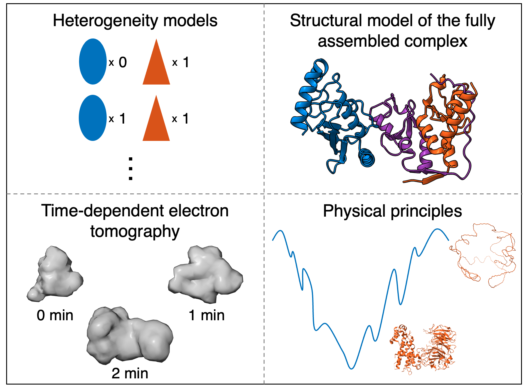
The heterogeneity models inform protein copy numbers for the snapshot models. The PDB structure of the complex informs the structure of the individual proteins. The time-dependent ET data informs the size and shape of the assembling complex. Physical principles inform connectivity and excluded volume.
Next, we represent, score and search for snapshot models. To do so, navigate to the Snapshots/Snapshots_Modeling/ folder. Here, you will find two python scripts. The first, static_snapshot.py, uses IMP to represent, score, and search for a single static snapshot model. The second, start_sim.py, automates the creation of a snapshot model for each heterogeneity model.
Here, we will describe the process of modeling a single snapshot model, as performed by running static_snapshot.py.
We begin by representing the data and the model. In general, the representation of a system is defined by all the variables that need to be determined.
For our model of a protein complex, we use a combination of two representations. The first is a series of spherical beads, which can correspond to portions of the biomolecules of interest, such as atoms or groups of atoms. The second is a series of 3D Gaussians, which help calculate the overlap between our model and the density from ET data.
Beads and Gaussians in our model belong to either a rigid body or flexible string. The positions of all beads and Gaussians in a single rigid body are constrained during sampling and do not move relative to each other. Meanwhile, flexible beads can move freely during sampling, but are restrained by sequence connectivity.
To begin, we built a topology file with the representation for the model of the complete system, spatiotemporal_topology.txt, located in Heterogeneity/Heterogeneity_Modeling/. This complete topology was used as a template to build topologies of each snapshot model. Based on our observation of the structure of the complex, we chose to represent each protein with at least 2 separate rigid bodies, and left the first 28 residues of protein C as flexible beads. Rigid bodies were described with 1 bead for every residue, and 10 residues per Gaussian. Flexible beads were described with 1 bead for every residue and 1 residue per Gaussian. A more complete description of the options available in topology files is available in the the TopologyReader documentation.
Next, we must prepare static_snapshot.py to read in this topology file. We begin by defining the input variables, state and time, which define which heterogeneity model to use, as well as the paths to other pieces of input information.
Next, we build the system, using the topology tile, described above.
Then, we prepare for later sampling steps by setting which Monte Carlo moves will be performed. Rotation (rot) and translation (trans) parameters are separately set for super rigid bodies (srb), rigid bodies (rb), and beads (bead).
After building the model representation, we choose a scoring function to score the model based on input information. This scoring function is represented as a series of restraints that serve as priors.
We begin with a connectivity restraint, which restrains beads adjacent in sequence to be close in 3D space.
Next is an excluded volume restraint, which restrains beads to minimize their spatial overlap.
Finally, we restrain our models based on their fit to ET density maps. Both the experimental map and the forward protein density are represented as Gaussian mixture models (GMMs) to speed up scoring. The score is based on the log of the correlation coefficient between the experimental density and the forward protein density.
After building a scoring function that scores alternative models based on their fit to the input information, we aim to search for good scoring models. For complicated systems, stochastic sampling techniques such as Monte Carlo (MC) sampling are often the most efficient way to compute good scoring models. Here, we generate a random initial configuration and then perform temperature replica exchange MC sampling with 16 temperatures from different initial configurations. By performing multiple runs of replica exchange MC from different initial configurations, we can later ensure that our sampling is sufficiently converged.
After performing sampling, a variety of outputs will be created. These outputs include .rmf files, which contain multi-resolution models output by IMP, and .out files which contains a variety of information about the run such as the value of the restraints and the MC acceptance rate.
Next, we will describe the process of computing multiple static snapshot models, as performed by running start_sim.py.
From heterogeneity modeling, we see that there are 3 heterogeneity models at each time point (it is possible to have more snapshot models than copy numbers if multiple copies of the protein exist in the complex), each of which has a corresponding topology file in Heterogeneity/Heterogeneity_Modeling/. We wrote a function, generate_all_snapshots, which creates a directory for each snapshot model, copies the python script and topology file into that directory, and submits a job script to run sampling. The job script will likely need to be customized for the user's computer or cluster.
We note that sometimes errors such as the one below can arise during sampling. These errors are caused by issues generating forward GMM files, which is done stochastically. If such issues arrise, remove all files in the forward_densities folder for that snapshot model and resubmit the corresponding jobs.
Now, we have a variety of alternative snapshot models. In general, we would like to assess these models in at least 4 ways: estimate the sampling precision, compare the model to data used to construct it, validate the model against data not used to construct it, and quantify the precision of the model. Here, we will focus specifically on estimating the sampling precision of the model, while quantitative comparisons between the model and experimental data will be reserved for the final step, when we assess trajectories. To assess these snapshot models, we navigate to the Snapshots/Snapshots_Assessment folder and run snapshot_assessment.py. This script performs the following analysis.
Initially, we want to filter the various alternative structural models to only select those that meet certain parameter thresholds. In this case, we filter the structural models comprising each snapshot model by the median cross correlation with EM data. We note that this filtering criteria is subjective, and developing a Bayesian method to objectively weigh different restraints for filtering remains an interesting future development in integrative modeling.
The current filtering procedure involves three steps. In the first step, we look through the stat.*.out files to write out the cross correlation with EM data for each model, which, in this case, is labeled column 3, GaussianEMRestraint_None_CCC. In other applications, the column that corresponds to each type of experimental data may change, depending on the scoring terms for each model. For each snapshot model, a new file is written with this data ({state}_{time}_stat.txt).
In the second step, we want to determine the median value of EM cross correlation for each snapshot model. We wrote general_rule_calculation to look through the general_rule_column for each {state}_{time}_stat.txt file and determine both the median value and the number of structures generated.
In the third step, we use the imp_sampcon select_good tool to filter each snapshot model, according to the median value determined in the previous step. For each snapshot model, this function produces a file, good_scoring_models/model_ids_scores.txt, which contains the run, replicaID, scores, and sampleID for each model that passes filtering. It also saves RMF files with each model from two independent groups of sampling runs from each snapshot model to good_scoring_models/sample_A and good_scoring_models/sample_B, writes the scores for the two independent groups of sampling runs to good_scoring_models/scoresA.txt and good_scoring_models/scoresB.txt, and writes good_scoring_models/model_sample_ids.txt to connect each model to its division of sampling run. More information on imp_sampcon is available in the analysis portion of the actin tutorial.
Next, scores can be plotted for analysis. Here, we wrote the create_histograms function to run imp_sampcon plot_score so that it plots distributions for various scores of interest. Each of these plots are saved to histograms{state}_{time}/{score}.png, where score is an object listed in the score_list. These plots are useful for debugging the modeling protocol, and should appear roughly Gaussian.
We then check the number of models in each sampling run though our function, count_rows_and_generate_report, which writes the independent_samples_stat.txt file. Empirically, we have found that ensuring the overall number of models in each independent sample after filtering is roughly equal serves a good first check on sampling convergence.
Next, we write the density range dictionaries, which are output as {state}_{time}_density_ranges.txt. These dictionaries label each protein in each snapshot model, which will be passed into imp_sampcon to calculate the localization density of each protein.
Next, we run imp_sampcon exhaust on each snapshot model. This code performs checks on the exhaustiveness of the sampling. Specifically it analyzes the convergence of the model score, whether the two model sets were drawn from the same distribution, and whether each structural cluster includes models from each sample proportionally to its size. The output for each snapshot model is written out to the exhaust_{state}_{time} folder.
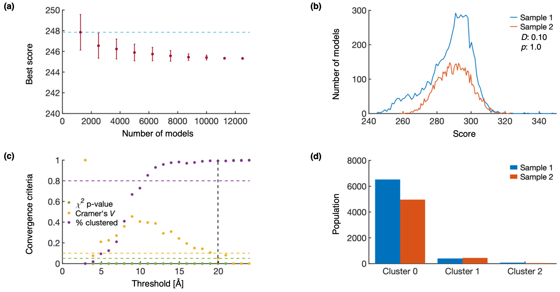
Plots for determining the sampling precision are shown below for a single snapshot model, 1_2min. (a) Tests the convergence of the lowest scoring model (snapshot_{state}_{time}.Top_Score_Conv.pdf). Error bars represent standard deviations of the best scores, estimated by selecting 150 different subsets of models. The light-blue line helps compare the highest average top score to the top score from other subsets of models. (b) Tests that the scores of two independently sampled models come from the same distribution (snapshot_{state}_{time}.Score_Dist.pdf). The difference between the two distributions, as measured by the KS test statistic (D) and KS test p-value (p) indicates that the difference is both statistically insignificant (p>0.05) and small in magnitude (D<0.3). (c) Determines the structural precision of a snapshot model (snapshot_{state}_{time}.ChiSquare.pdf). RMSD clustering is performed at 1 Å intervals until the clustered population (% clustered) is greater than 80%, and either the χ2 p-value is greater than 0.05 or Cramer’s V is less than 0.1. The sampling precision is indicated by the dashed black line. (d) Populations from sample 1 and sample 2 are shown for each cluster (snapshot_{state}_{time}.Cluster_Population.pdf).
Further structural analysis can be calculated by using the cluster.* files. The cluster.*.{sample}.txt files contain the model number for the models in that cluster, where {sample} indicates which round of sampling the models came from. The cluster.* folder contains an RMF for centroid model of that cluster, along with the localization densities for each protein. The localization densities of each protein from each independent sampling can be compared to ensure independent samplings produce the same results.
Ideally, each of these plots should be checked for each snapshot model. As a way to summarize the output of these checks, we can gather the results of the KS test and the sampling precision test for all snapshot models. This is done by running extract_exhaust_data and save_exhaust_data_as_png, which write KS_sampling_precision_output.txt and KS_sampling_precision_output.png, respectively.
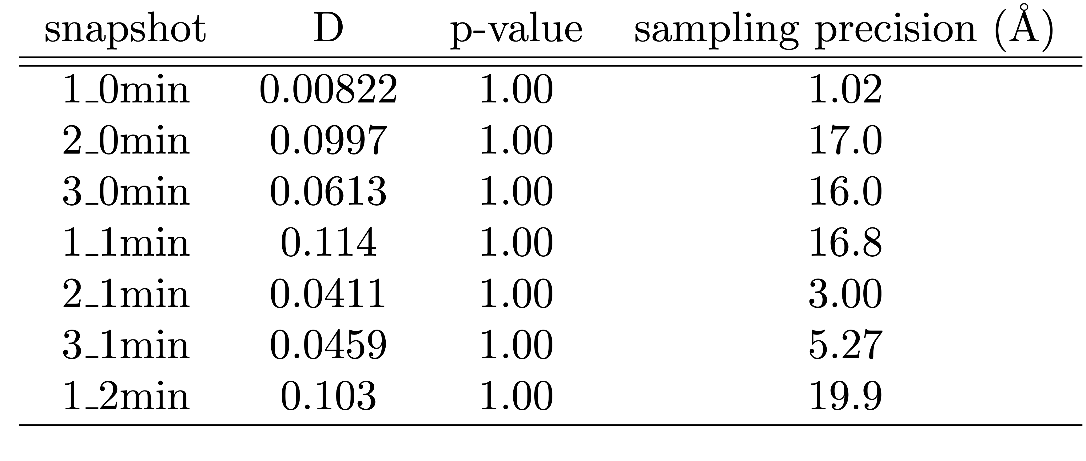
These codes write a table that include the KS two sample test statistic (D), the KS test p-value, and the sampling precision for each snapshot model, which is replotted below.
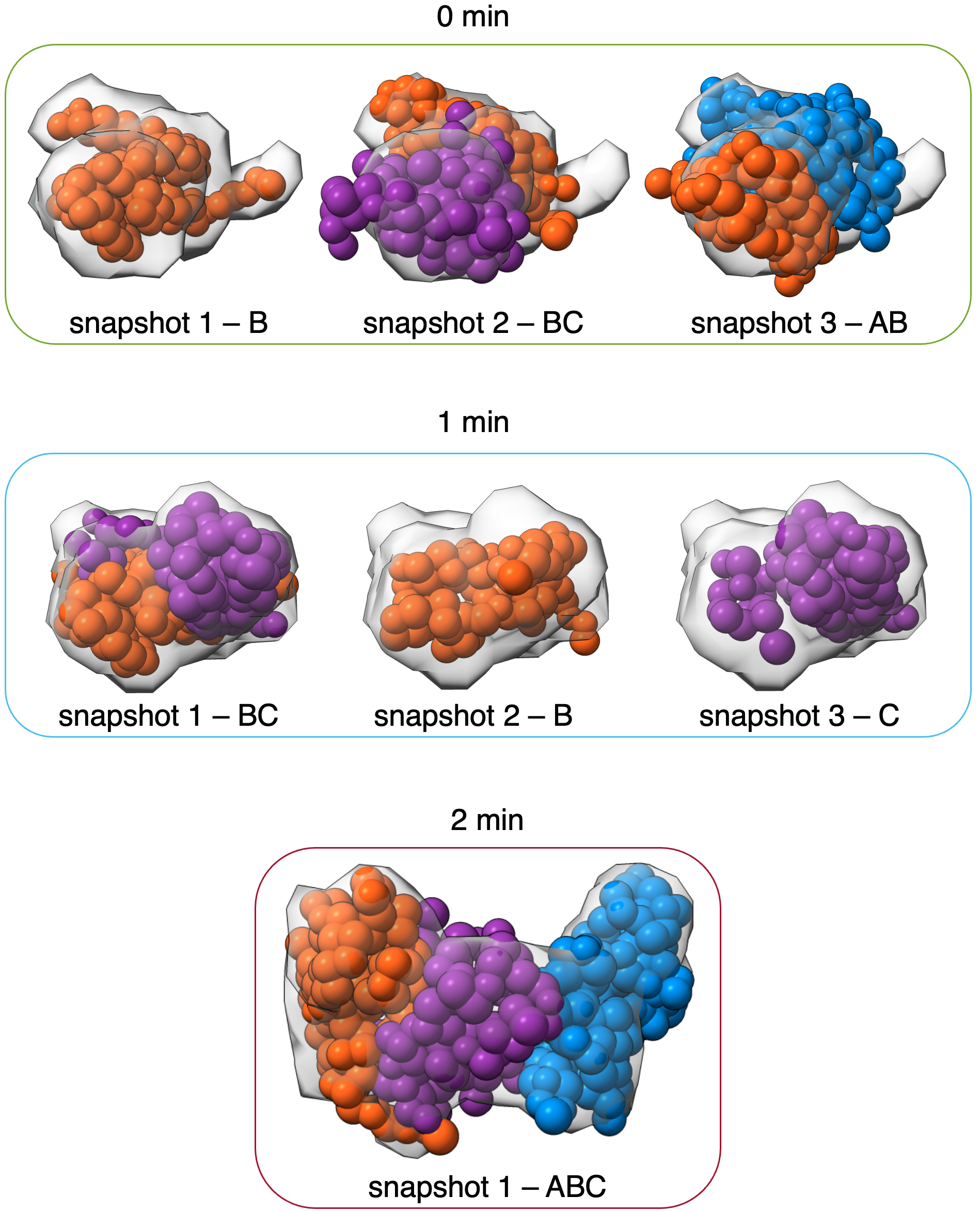
The resulting RMF files and localization densities from this analysis can be viewed in UCSF Chimera (version>=1.13) or UCSF ChimeraX.
Here, we plotted each centroid model (A - blue, B - orange, and C - purple) from the most populated cluster for each snapshot model and compared that model to the experimental EM profile (gray).
Finally, now that snapshot models have been assessed, we can perform Modeling of a trajectory.