 |
|
Integrative spatiotemporal modeling in IMP
|
Here, we describe the final modeling problem in our composite workflow, how to build a trajectory model using IMP.
We begin trajectory modeling with the first step of integrative modeling, gathering information. Trajectory modeling utilizes dynamic information about the bimolecular process. In this case, we utilize snapshot models, physical theories, and synthetically generated small-angle X-ray scattering (SAXS) profiles.
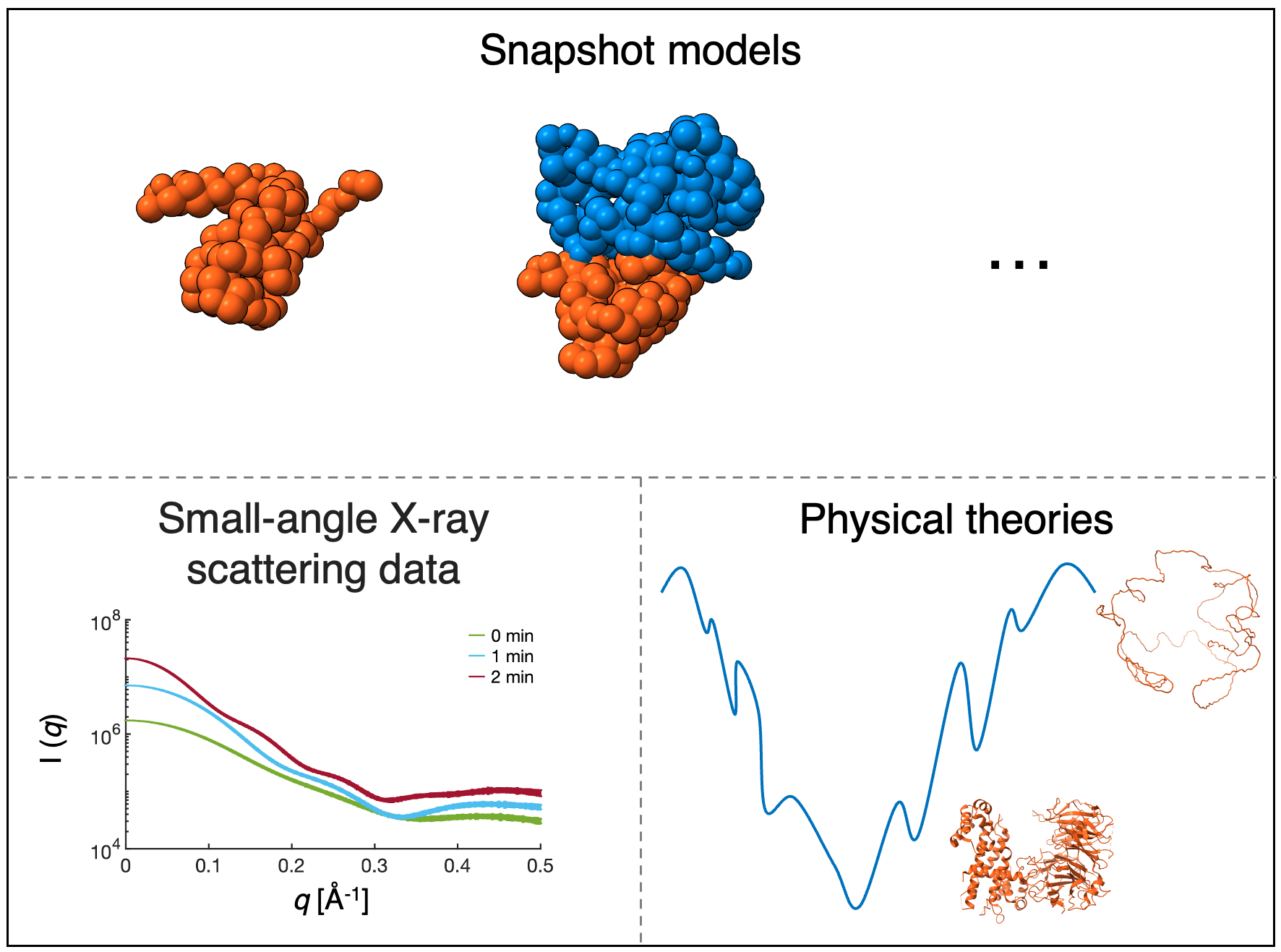
Snapshot models inform transitions between sampled time points, and their scores inform trajectory scores. Physical theories of macromolecular dynamics inform transitions between sampled time points. SAXS data informs the size and shape of the assembling complex and is left for validation.
Trajectory modeling connects alternative snapshot models at adjacent time points, followed by scoring the trajectories based on their fit to the input information, as described in full here.
We choose to represent dynamic processes as a trajectory of snapshot models, with one snapshot model at each time point. In this case, we computed snapshot models at 3 time points (0, 1, and 2 minutes), so a single trajectory will consist of 3 snapshot models, one at each 0, 1, and 2 minutes. The modeling procedure described here will produce a set of scored trajectories, which can be displayed as a directed acyclic graph, where nodes in the graph represent the snapshot model and edges represent connections between snapshot models at neighboring time points.
To score trajectories, we incorporate both the scores of individual snapshot models, as well as the scores of transitions between them. Under the assumption that the process is Markovian (i.e. memoryless), the weight of a trajectory takes the form:
\[ W(\chi) \propto \displaystyle\prod^{T}_{t=0} P( X_{t} | D_{t}) \cdot \displaystyle\prod^{T-1}_{t=0} W(X_{t+1} | X_{t},D_{t,t+1}) \]
where \(t\) indexes times from 0 until the final modeled snapshot ( \(T\)); \(P(X_{t} | D_{t})\) is the snapshot model score; and \(W(X_{t+1} | X_{t}, D_{t,t+1})\) is the transition score. Trajectory weights ( \(W(\chi)\)) are normalized so that the sum of all trajectory weights is 1.0. Transition scores are currently based on a simple metric that either allows or disallows a transition. Transitions are only allowed if all proteins in the first snapshot model are included in the second snapshot model. In the future, we hope to include more detailed transition scoring terms, which may take into account experimental information or physical models of macromolecular dynamics.
Trajectories are constructed by enumerating all connections between adjacent snapshot models and scoring these trajectories according to the equation above. This procedure results in a set of weighted trajectories.
Navigate to Trajectories/Trajectories_Modeling. The create_trajectories.py script runs the above steps to create a spatiotemporal integrative model from the previously sampled snapshot models.
First, we copy all relevant files to a new directory, data. These files are (i) {state}_{time}.config files, which include the subcomplexes that are in each state, (ii) {state}_{time}_scores.log, which is a list of all scores of all structural models in that snapshot model, and (iii) exp_comp{prot}.csv, which is the experimental copy number for each protein ({prot}) as a function of time.
We then build the spatiotemporal graph by running spatiotemporal.create_DAG, documented here. This function represents, scores, and searches for trajectories.
The inputs we included are:
{state}_{time}.config files..csv file with the copy number data for that protein.After running spatiotemporal.create_DAG, a variety of outputs are written:
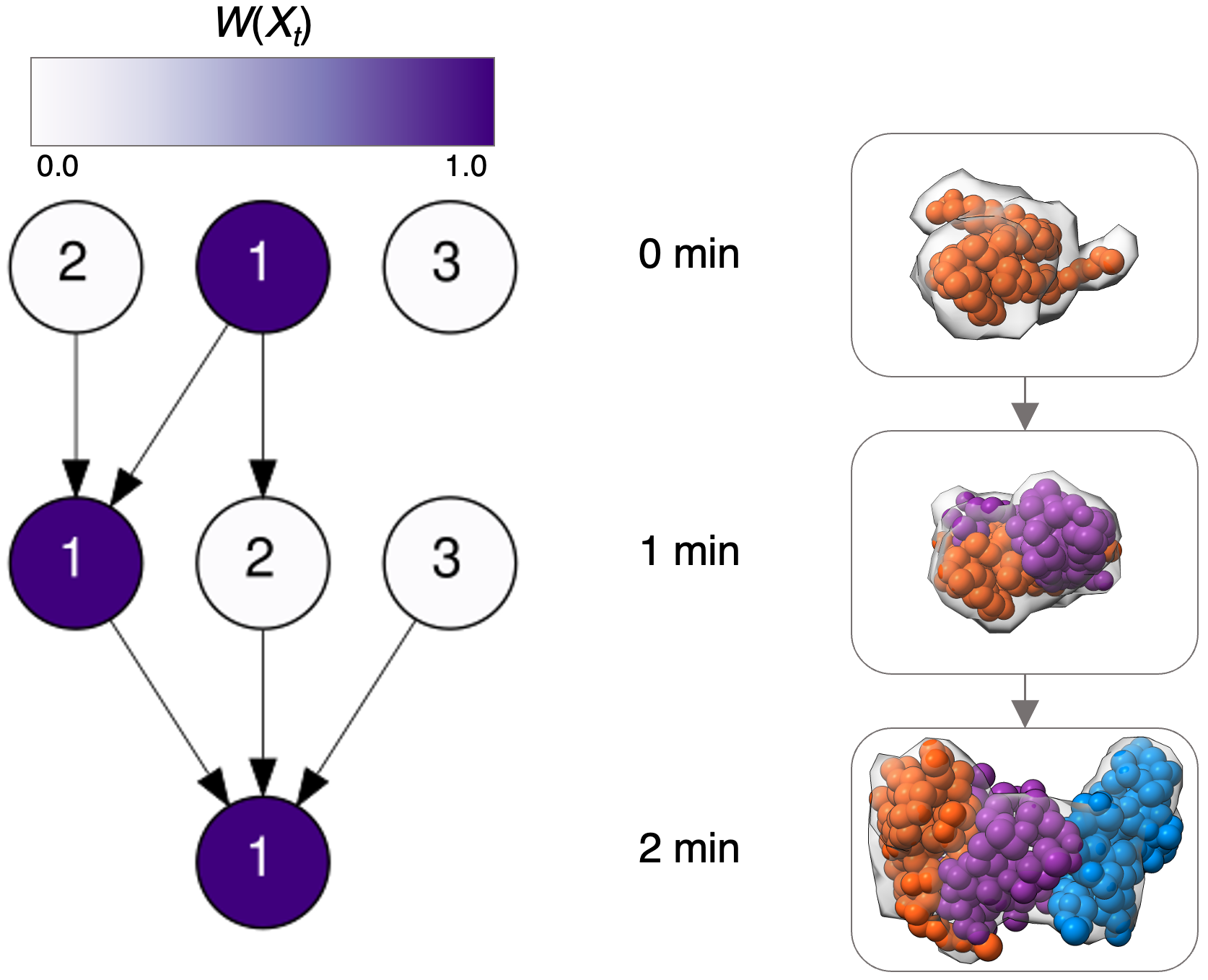
cdf.txt: the cumulative distribution function for the set of trajectories.pdf.txt: the probability distribution function for the set of trajectories.labeled_pdf.txt: Each row has 2 columns and represents a different trajectory. The first column labels a single trajectory as a series of snapshot models, where each snapshot model is written as {state}_{time}| in sequential order. The second column is the probability distribution function corresponding to that trajectory.dag_heatmap.eps and dag_heatmap: image of the directed acyclic graph from the set of trajectories.path*.txt: files where each row includes a {state}_{time} string, so that rows correspond to the states visited over that trajectory. Files are numbered from the most likely path to the least likely path.Now that we have a trajectory model, we can plot the directed acyclic graph (left) and the series of centroid models from each snapshot model along the most likely trajectory (right). Each row corresponds to a different time point in the assembly process (0 min, 1 min, and 2 min). Each node is shaded according to its weight in the final model ( \(W(X_{t})\)). Proteins are colored as A - blue, B - orange, and C - purple.
Now that the set of spatiotemporal models has been constructed, we must evaluate these models. We can evaluate these models in at least 4 ways: estimating the sampling precision, comparing the model to data used to construct it, validating the model against data not used to construct it, and quantifying the precision of the model.
Navigate to Trajectories/Trajectories_Assessment and run trajectories_assessment.py. This code will perform the following steps to assess the model.
To begin, we calculate the sampling precision of the models. The sampling precision is calculated by using spatiotemporal.create_DAG to reconstruct the set of trajectories using 2 independent sets of samplings for snapshot models. Then, the overlap between these snapshot models is evaluated using analysis.temporal_precision, which takes in two labeled_pdf files.
The output of analysis.temporal_precision is written in analysis_output_precision/temporal_precision.txt, shown below. The temporal precision can take values between 1.0 and 0.0, and indicates the overlap between the two models in trajectory space. Hence, values close to 1.0 indicate a high sampling precision, while values close to 0.0 indicate a low sampling precision. Here, the value close to 1.0 indicates that sampling does not affect the weights of the trajectories.
Next, we calculate the precision of the model, using analysis.precision. Here, the model precision calculates the number of trajectories with high weights. The precision ranges from 1.0 to 1/d, where d is the number of trajectories. Values approaching 1.0 indicate the model set can be described by a single trajectory, while values close to 1/d indicate that all trajectories have similar weights.
The analysis.precision function reads in the labeled_pdf of the complete model, and writes the output file to analysis_output_precision/precision.txt, shown below. The value close to 1.0 indicates that the set of models can be sufficiently represented by a single trajectory.
We then evaluate the model against data used in model construction. First, we calculate the cross-correlation between the original EM map and the forward density projected from each snapshot model. We wrote the ccEM function to perform this comparison for all snapshot models.
The output of ccEM is written in ccEM_output/. It contains forward densities for each snapshot model (MRC_{state}_{time}.mrc) and ccEM_calculations.txt, which contains the cross-correlation to the experimental EM profile for each snapshot model.
After comparing the model to EM data, we aimed to compare the model to copy number data, and wrote the forward_model_copy_number function to evaluate the copy numbers from our set of trajectories.
The output of forward_model_copy_number is written in forward_model_copy_number/. The folder contains CN_prot_{prot}.txt files for each protein, which have the mean and standard deviation of protein copy number at each time point.
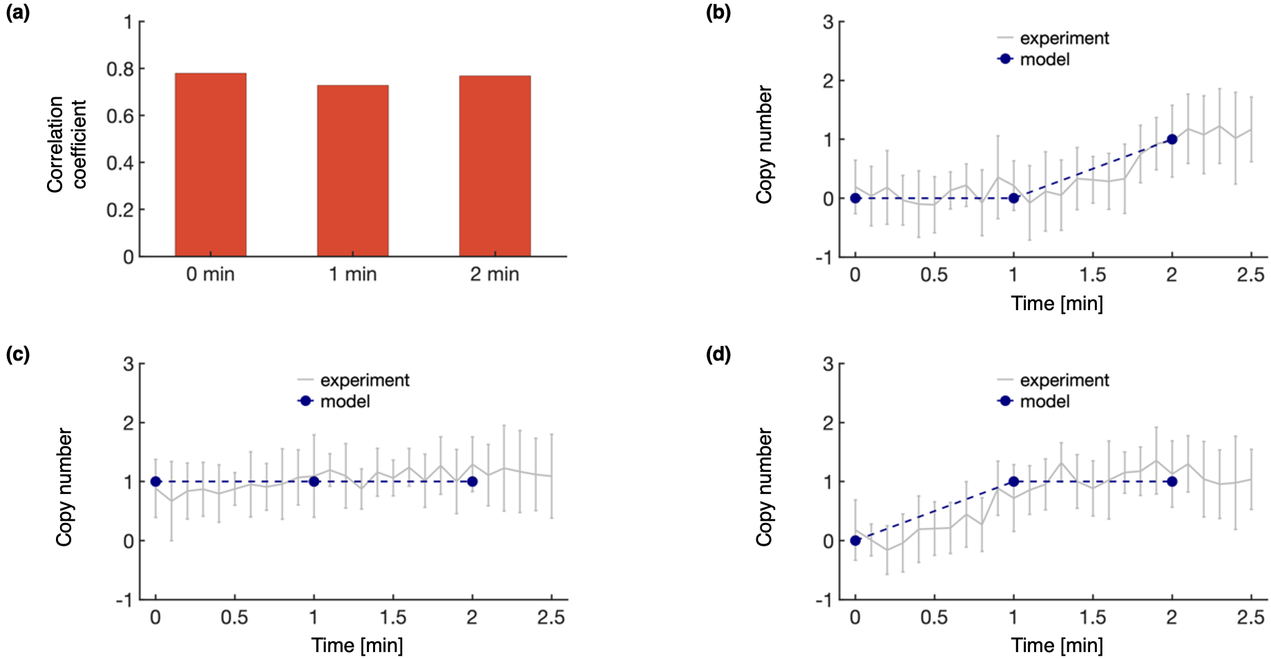
Here, we plot the comparison between the experimental data used in model construction and the set of trajectories. This analysis includes the cross-correlation coefficient between the experimental EM density and the forward density of the set of sufficiently good scoring modeled structures in the highest weighted trajectory (a), as well as comparisons between experimental and modeled protein copy numbers for proteins A (b), B (c), and C (d). Here, we see the model is in good agreement with the data used to construct it.
Finally, we aim to compare the model to data not used in model construction. Specifically, we reserved SAXS data for model validation. We aimed to compare the forward scattering profile from the centroid structural model of each snapshot model to the experimental profile. To make this comparison, we wrote functions that converted each centroid RMF to a PDB (convert_rmfs), copied the experimental SAXS profiles to the appropriate folder (copy_SAXS_dat_files), and ran FoXS on each PDB to evaluate its agreement to the experimental profile (process_foxs).
The output of this analysis is written to SAXS_comparison. Standard FoXS outputs are available for each snapshot model (snapshot{state}_{time}.*). In particular, the .fit files include the forward and experimental profiles side by side, with the \(\chi^2\) for the fit. Further, the {time}_FoXS.* files include the information for all snapshot models at that time point, including plots of each profile in comparison to the experimental profile ({time}_FoXS.png).
As our model was generated from synthetic data, the ground truth structure is known at each time point. In addition to validating the model by assessing its comparison to SAXS data, we could approximate the model accuracy by comparing the snapshot model to the PDB structure, although this comparison is not perfect as the PDB structure was used to inform the structure of rigid bodies in the snapshot model. To do so, we wrote a function (RMSD) that calculates the RMSD between each structural model and the orignal PDB.
The output of this function is written in RMSD_calculation_output. The function outputs rmsd_{state}_{time}.png files, which plots the RMSD for each structural model within each snapshot model. This data is then summarized in RMSD_analysis.txt, which includes the minimum RMSD, average RMSD, and number of structural models in each snapshot model.
Here, we plot the results for assessing the spatiotemporal model with data not used to construct it. Comparisons are made between the centroid structure of the most populated cluster in each snapshot model at each time point and the experimental SAXS profile for 0 (a), 1 (b), and 2 (c) minutes. Further, we plot both the sampling precision (dark red) and the RMSD to the PDB structure (light red) for each snapshot model in the highest trajectory (d).
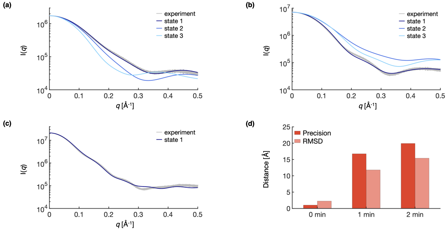
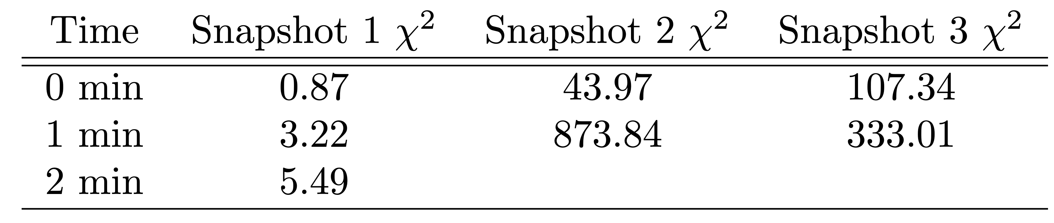
To quantitatively compare the model to SAXS data, we used the \(\chi^2\) to compare each snapshot model to the experimental profile. We note that the \(\chi^2\) are substantially lower for the models along the highest trajectory (1_0min, 1_1min, and 1_2min) than for other models, indicating that the highest weighted trajectory is in better agreement with the experimental SAXS data than other possible trajectories.
Next, we can evaluate the accuracy of the model by comparing the RMSD to the PDB to the sampling precision of each snapshot model. We note that this is generally not possible, because in most biological applications the ground truth is not known. In this case, if the average RMSD to the PDB structure is smaller than the sampling precision, the PDB structure lies within the precision of the model. We find that the RMSD is within 1.5 Å of the sampling precision at all time points, indicating that the model lies within 1.5 Å of the ground truth.
After assessing our model, we can must decide if the model is sufficient to answer biological questions of interest. If the model does not have sufficient precision for the desired application, assessment of the current model can be used to inform which new experiments may help improve the next iteration of the model. The integrative spatiotemporal modeling procedure can then be repeated iteratively, analogous to integrative modeling of static structures.
If the model is sufficient to provide insight into the biological process of interest, the user may decide that it is ready for publication. In this case, the user should create an mmCIF file to deposit the model in the PDB-IHM database. This procedure is explained in the deposition tutorial.