 |
|
Integrative spatiotemporal modeling in IMP
|
Biomolecules are constantly in motion; therefore, a complete depiction of their function must include their dynamics instead of just static structures. We have developed an integrative spatiotemporal approach to model dynamic systems.
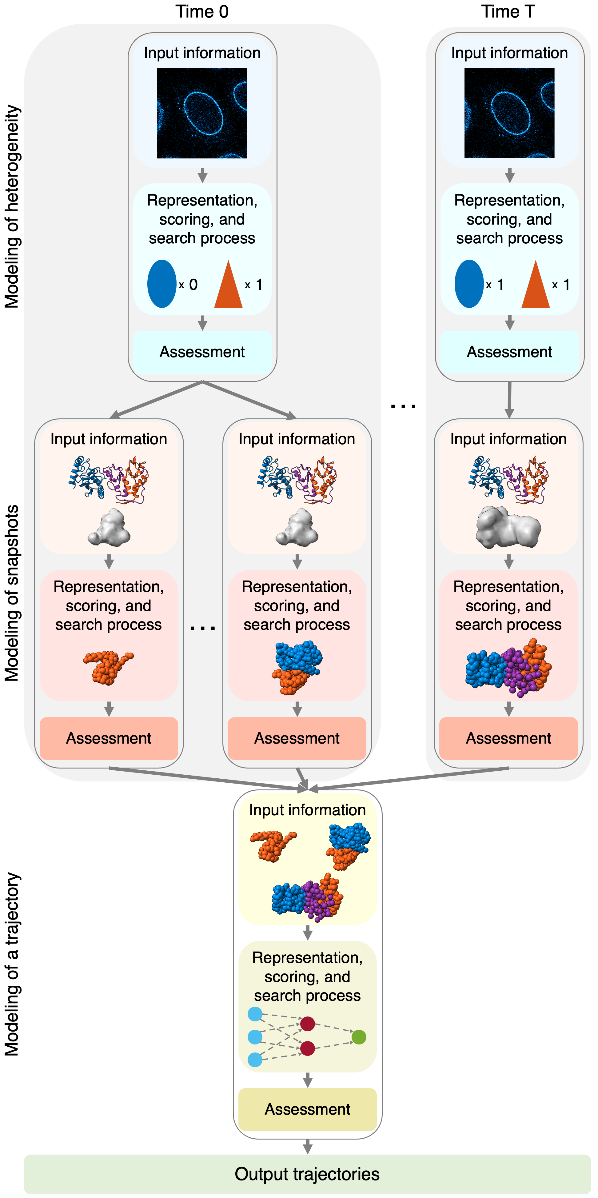
Our approach applies a composite workflow, consisting of three modeling problems to compute (i) heterogeneity models, (ii) snapshot models, and (iii) a trajectory model. Heterogeneity models describe the possible biomolecular compositions of the system at each time point. Optionally, other auxiliary variables can be considered, such as the coarse location in the final state when modeling an assembly process. For each heterogeneity model, one snapshot model is produced. A snapshot model is a set of alternative standard static integrative structure models based on the information available for the corresponding time point. Then, a set of trajectories ranked by their agreement with input information is computed by connecting alternative snapshot models at adjacent time points (i.e., the “trajectory model”). This trajectory model can be scored based on both the scores of static structures and the transitions between them, allowing for the creation of trajectories that are in agreement with the input information by construction.
If you use this tutorial or its accompanying method, please cite the corresponding publications:
In general, integrative modeling proceeds through three steps (i. gathering information; ii. choosing the model representation, scoring alternative models, and searching for good scoring models; and iii. assessing the models). In integrative spatiotemporal modeling, these three steps are repeated for each modeling problem in the composite workflow (i. modeling of heterogeneity, ii. modeling of snapshots, and iii. modeling of a trajectory).

This tutorial will walk you through the links below, which contain a breakdown of each of these modeling steps for the hypothetical assembly mechanism of the Bmi1/Ring1b-UbcH5c complex. We note that all experimental data besides the static structure used in this study is purely hypothetical, and, thus, the model should not be interpreted to be meaningful about the actual assembly mechanism of the complex.
To work through this example, a variety of python packages will be necessary in addition to IMP. These packages are numpy, os, warnings, sys, itertools, pandas, matplotlib, pyRMSD, and graphviz. Optionally, UCSF Chimera, UCSF ChimeraX, gnuplot, and MATLAB can be used for visualizing structures or plotting data.
The code for this tutorial is available through its GitHub link. A complete, worked example of the tutorial is available in the modeling folder; meanwhile, the necessary code and input information without the resulting model are available in the modeling_empty folder, from which the user can run the code for themselves. A Google Colab notebook with the less computationally expensive steps is also available.
Our tutorial begins by modeling the heterogeneity of the system.