 |
|
Modeling of an actin complex with PMI
|
Analysis is performed using the IMP.sampcon module. The already-generated sampling output will be analyzed here; it is contained in the compressed files run1.zip and run2.zip in the modeling folder (they should first be extracted to make modeling/run1 and modeling/run2).
Analysis is performed in a new directory: analysis/tutorial_analysis.
The imp_sampcon select_good tool filters models based on score and parameter thresholds. In this tool, required flags are: -rd, which specifies the directory containing sampling output folders; -rp, which defines the prefix for the sampling output folders; -sl, which defines the stat file keywords (see below) that we wish to filter on; -pl, which specifies the keywords that will be written to the output file; -alt and -aut, which specify, respectively, the lower and upper threshold for each keyword in -slt that define acceptance. The -mlt and -mut keywords, which are optional, define thresholds for restraints made of multiple components (such as crosslinks).
imp_sampcon show_stat ./path/to/stat/fileHere, we first use crosslink satisfaction as an initial filtering criterion because we usually have an a priori estimate of the false positive rate and/or cutoff distance (for scores whose thresholds are not known a priori, one can perform a multi-stage filtering process as outlined in the above protocol). For this simulated system, we only accept models with 100% satisfaction of crosslinks by setting both -alt and -aut to 1.0. A crosslink is satisfied if the distance is between 0.0 and 30.0 Å, as delineated by the -mlt and -mut keywords, respectively. We specify that connectivity, crosslink data score, excluded volume, EM, SAXS and total scores be printed as well.
This script creates a directory filter and a file, filter/model_ids_scores.txt, that contains the model index, its run, replicaID, frame ID, scores, and sample ID for each model. We can now use the script plot_score.py to plot the distribution of SAXS, EM, connectivity and excluded volume scores from this first set of filtered models to determine a reasonable threshold for accepting or rejecting a model.
The resulting histograms (SAXSRestraint_score.png and GaussianEMRestraint_None.png) are roughly Gaussian. Based on these distributions we set our criteria for good scoring models as those whose EM and SAXS scores are >1 standard deviation below the mean, except for connectivity, which is well satisfied in almost all models and EM, which has a large tail. Our high score thresholds are -7.0 for EM, and 0.3 for SAXS, 1.0 for connectivity and 4.916 for excluded volume.
We rerun imp_sampcon select_good adding the extra keywords and score thresholds. We add the extra flag, -e, to extract Rich Molecular Format (RMF) files of all good scoring models. These thresholds return 1582 good scoring models.
The output directory, good_scoring_models, contains folders sample_A and sample_B, which hold the RMF files of the good scoring models for each independent run (or set of runs). The file model_ids_scores.txt contains the model index, its run, replicaID, frame ID, scores, and sample ID for each model.
The imp_sampcon exhaust tool is used to calculate the sampling precision at which the modeling is exhaustive. During this step, multiple tests for convergence are performed on the two samples determined above, models are clustered, and localization densities are computed.
First, we create a file, density_ranges.txt, in the tutorial_analysis directory with a single line that defines components using PMI selection tuples on which we calculate localization densities. Here, we create three localization densities, one for the entire actin molecule and one each for the structured residues of each of the other two molecules.
We now run the command for testing sampling exhaustiveness.
The system name, actin, defines the labels for the output files.
The -a flag aligns all models (alignment of models is sometimes not necessary, e.g. when one has a medium resolution or better EM map).
The -g flag determines the step size in Å for calculating sampling precision. (This is the step size at which clustering is performed between the minimum and maximum RMSDs in the dataset. This tutorial uses 0.1Å to get a very precise estimate of the sampling precision; however this results in a very long calculation. In practice, especially for larger systems whose sampling precision will be much lower, one would choose a larger value to make calculation more efficient.)
This routine can be run in parallel using the -m cpu_omp flag and -c N, where N is the number of processors. (If alignment is necessary, the GPU mode of pyRMSD generally increases performance significantly. It is invoked by using -m cuda.)
The -p flag defines the path to the good scoring model directory.
The results of the convergence tests are summarized in the output figure, actin_convergence.png, below, which identifies our sampling precision of 3.5Å, with one dominant cluster, one minor cluster and one cluster of insignificant size. Text files containing this information are also produced. (The output of the protocol can be readily plotted using any plotting software. Scripts for gnuplot are included in the IMP distribution; print ‘IMP.sampcon.get_data_path('gnuplot_scripts’)from a Python interpreter to find the folder containing them, or add–gnuplotto the imp_sampcon exhaust` invocation to automatically run them at the end of the protocol.)
Output also includes localization densities for each cluster, which are contained in separate directories (cluster.0, cluster.1, ...). Within these directories are a representative RMF file cluster_center_model.rmf3 and localization densities for each subunit defined in the density_ranges.txt file.
-s) along with the value of clustering threshold (-ct) allows one to bypass RMSD and sampling precision calculation and get the clusters and their densities, as follows: imp_sampcon exhaust -n actin -d density_custom.txt -ct 4.39 -a -s. Note that this clustering threshold should always be worse than the sampling precision.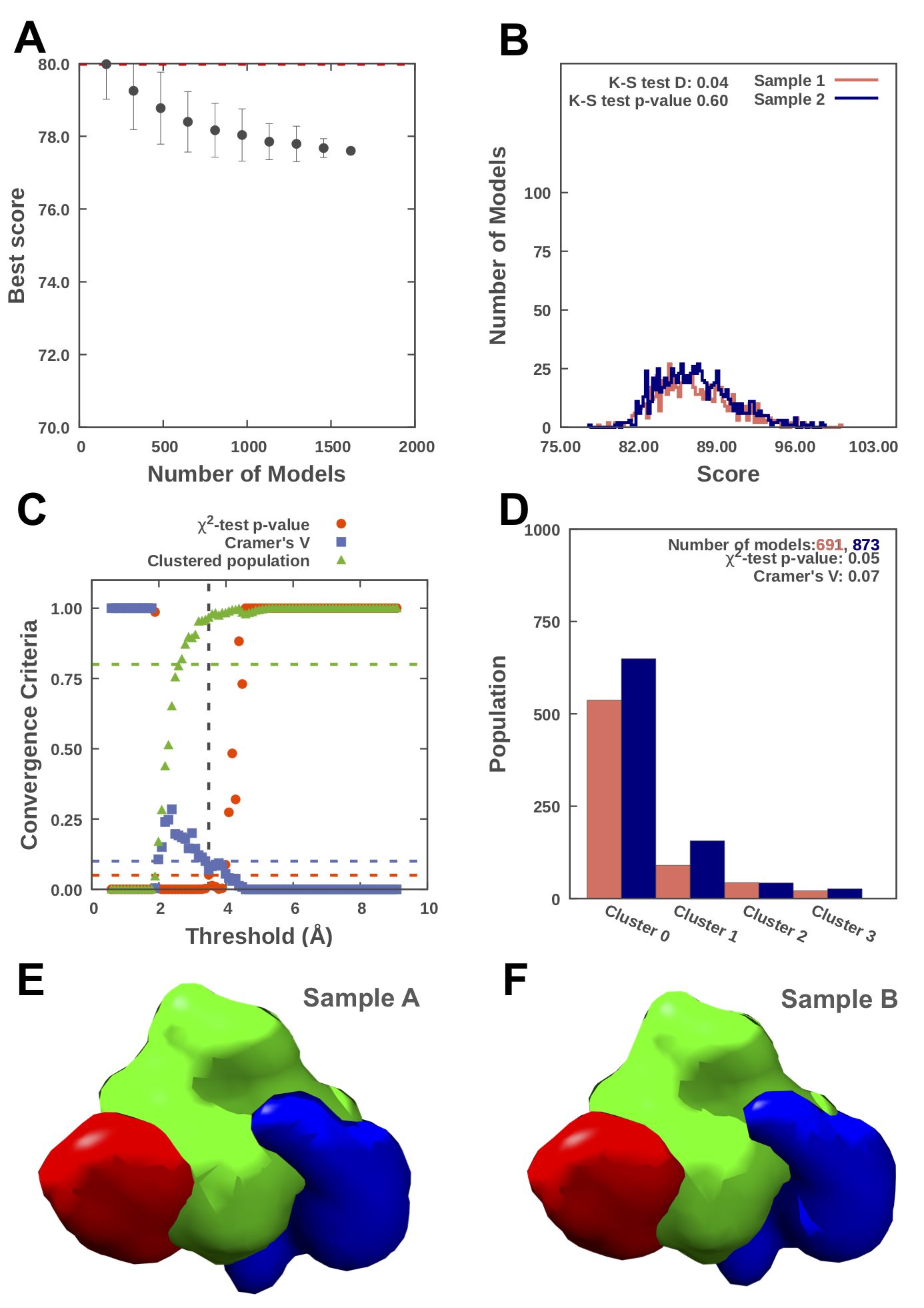
Results for sampling exhaustiveness protocol for modeling in complex of actin and tropomodulin-gelsolin chimera. A. Results of test 1, convergence of the model score, for the 1618 good-scoring models; the scores do not continue to improve as more models are computed essentially independently. The error bar represents the standard deviations of the best scores, estimated by repeating sampling of models 150 times. The red dotted line indicates a lower bound reference on the total score. B. Results of test 2, testing similarity of model score distributions between samples 1 (red) and 2 (blue); the difference in distribution of scores is significant (Kolmogorov-Smirnov two-sample test p-value less than 0.05) but the magnitude of the difference is small (the Kolmogorov-Smirnov two-sample test statistic D is 0.02); thus, the two score distributions are effectively equal. C. Results of test 3, three criteria for determining the sampling precision (Y-axis), evaluated as a function of the RMSD clustering threshold (X-axis). First, the p-value is computed using the χ2-test for homogeneity of proportions (red dots). Second, an effect size for the χ2-test is quantified by the Cramer's V value (blue squares). Third, the population of models in sufficiently large clusters (containing at least 10 models from each sample) is shown as green triangles. The vertical dotted grey line indicates the RMSD clustering threshold at which three two conditions are satisfied (p-value > 0.05 [dotted red line], Cramer's V < 0.10 [dotted blue line], and the population of clustered models > 0.80 [dotted green line]), thus defining the sampling precision of 3.5Å (See an important note below for currently implemented criteria)*. D. Populations of sample 1 and 2 models in the clusters obtained by threshold-based clustering using the RMSD threshold of 3.5Å. Cluster precision is shown for each cluster. E. and F. Results of test 4: comparison of localization probability densities of models from sample A and sample B for the major cluster (84% population). The cross-correlation of the density maps of the two samples is 0.99 for the gelsolin (red) and tropomysin (blue) maps and 0.97 for the actin map (green).
NOTE: It's important to note that the protocol implementation for the BJ 2017 paper (at salilab.org/sampcon) is slightly different and more conservative than the current imp-sampcon implementation (at github.com/salilab/imp-sampcon). See the section "Minor updates to the protocol from the [BJ Paper](https://pubmed.ncbi.nlm.nih.gov/29211988) " in the README, related issues issue #39 and issue #5. Currently, the sampling precision defined here (github.com/salilab/imp-sampcon) is as follows: The minimum RMSD clustering threshold (vertical dotted line) at which both conditions are satisfied, i.e., Cramer's V < 0.10 [dotted blue line], and the population of clustered models > 0.80 [dotted green line].
The cluster RMF files and localization densities can be visualized using UCSF Chimera version >= 1.13, or UCSF ChimeraX with the RMF plugin (available from the ChimeraX toolshed). Example scripts for visualizing all localization densities are provided in the IMP distribution; print ‘IMP.sampcon.get_data_path('chimera_scripts’)` from a Python interpreter to find the folder containing them.
At this point, one must decide if the models are helpful in answering our biological questions. In the case of this tutorial, the PPI is localized to within a few Å and we can make predictions as to what residues may be important for this interaction. If our models are not well enough resolved, more information may have to be added through additional experiments, addition of constraints to the sampling, change in system representation, and/or additional sampling. We can iterate this process until we are satisfied with our output models.
Additional validation of the final model ensemble can be performed by rerunning the above protocol while omitting one or more of the input data points. Ideally, models generated with only a subset of the data will not differ significantly from the original models. Further, any information not used in the modeling process can be used as a validation of the final model ensemble, as discussed earlier.
For our modeling to be reproducible - a key requirement for the 4-stage modeling procedure and for science in general - the modeling protocol, all of the input data we used, and the final output models, should be deposited in a public location, ideally the PDB-IHM repository.
The modeling protocol includes the entire procedure of converting raw input data to output models, and so comprises both the set of IMP Python scripts described above and any procedures used to prepare IMP inputs, such as comparative modeling of subunits, segmentation of an EM density, and processing of XL-MS data to get a set of proximate residues. An excellent way to store and disseminate such a protocol is by using a source control system with a publicly accessible web frontend, such as GitHub (as is used for this tutorial). Integrative modeling is an inherently collaborative process. Source control makes it straightforward to track changes to all of the protocol scripts and data by local and remote collaborators. All protocol files should be deposited in a permanent location with a fixed Digital Object Identifier (DOI). A number of free services are available for deposition of such files, such as Zenodo and FigShare, where a snapshot of a GitHub repository for the published work can be deposited. For an example, see the previously-published modeling of Nup84.
Each piece of input data used should also be publicly available. Where possible, this data should be deposited in a repository specific to the given experimental technique and referenced from the model mmCIF file. For example, all of the crystal structures used in this example are simply referenced by their PDB IDs. Where such a repository does not exist, the data files should be made available at a DOI. The simplest way to archive these files is to store them in the same GitHub repository used for the modeling protocol. If derived data are used, the modeling protocol should indicate where the original raw data came from.
A decision needs to be made about which models to deposit. Generally, a representative sample of each cluster should be deposited, together with the localization densities of the entire cluster. The mmCIF file format allows for multiple models, potentially at multiple scales, in multiple states, and/or different time points, to be stored in a single file together with pointers to the input data and modeling protocol. Implementation of this format in IMP is still under development. The functionality will extract information from the RMF files output by the IMP modeling and combine it with metadata extracted from each experimental input. This file can be visualized in UCSF ChimeraX, and similar files from real modeling runs can be deposited in PDB-IHM and cited in publications.
