 |
|
PMI RNAPII Modeling Tutorial
|
In this stage, we will initially define a representation of the system. Afterwards, we will convert the data into spatial restraints. This is performed using the script rnapolii/modeling/modeling.py and uses the topology file, topology.txt, to define the system components and their representation parameters.
Representation
Very generally, the representation of a system is defined by all the variables that need to be determined based on input information, including the assignment of the system components to geometric objects (e.g. points, spheres, ellipsoids, and 3D Gaussian density functions).
Our RNA Pol II representation employs spherical beads of varying sizes and 3D Gaussians, which coarsen domains of the complex using several resolution scales simultaneously. The spatial restraints will be applied to individual resolution scales as appropriate.
Beads and Gaussians of a given domain are arranged into either a rigid body or a flexible string, based on the crystallographic structures. In a rigid body, all the beads and the Gaussians of a given domain have their relative distances constrained during configurational sampling, while in a flexible string the beads and the Gaussians are restrained by the sequence connectivity.
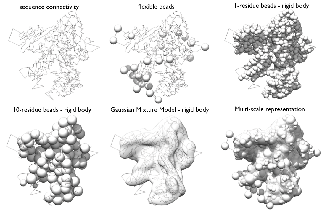
The GMM of a subunit is the set of all 3D Gaussians used to represent it; it will be used to calculate the EM score. The calculation of the GMM of a subunit can be done automatically in the topology file. For the purposes of this tutorial, we already created these for Rpb4 and Rpb7 and placed them in the rnapolii/data directory in their respective .mrc and .txt files.
Dissecting the script
The script rnapolii/modeling/modeling.py sets up the representation of the system and the restraint. (Subsequently it also performs sampling, but more on that later.)
Header
The first part of the script defines the files used in model building and restraint generation.
The first section defines where input files are located. The topology file defines how the system components are structurally represented. target_gmm_file stores the EM map for the entire complex, which has already been converted into a Gaussian mixture model.
Build the Model Representation Using a Topology File
Using the topology file we define the overall topology: we introduce the molecules with their sequence and their known structure, and define the movers. Each line in the file is a user-defined molecular Domain, and each column contains the specifics needed to build the system. See the TopologyReader documentation for a full description of the topology file format.
Building the System Representation and Degrees of Freedom
Here we can set the Degrees of Freedom parameters, which should be optimized according to MC acceptance ratios. There are three kind of movers: Rigid Body, Bead, and Super Rigid Body (super rigid bodies are sets of rigid bodies and beads that will move together in an additional Monte Carlo move).
max_rb_trans and max_rb_rot are the maximum translation and rotation of the Rigid Body mover, max_srb_trans and max_srb_rot are the maximum translation and rotation of the Super Rigid Body mover and max_bead_trans is the maximum translation of the Bead Mover.
The execution of the macro will return the root hierarchy (root_hier) and the degrees of freedom (dof) objects, both of which are used later on.
Since we're interested in modeling the stalk, we will fix all subunits except Rpb4 and Rpb7. Note that we are using IMP.atom.Selection to get the particles that correspond to the fixed Molecules.
Finally we randomize the initial configuration to remove any bias from the initial starting configuration read from input files. Since each subunit is composed of rigid bodies (i.e., beads constrained in a structure) and flexible beads, the configuration of the system is initialized by displacing each mobile rigid body and each bead randomly by 50 Angstroms, and rotate them randomly, and far enough from each other to prevent any steric clashes.
The excluded_rigid_bodies=fixed_rbs will exclude from the randomization everything that was fixed above.
After defining the representation of the model, we build the restraints by which the individual structural models will be scored based on the input data.
Connectivity Restraint
Excluded Volume Restraint
The excluded volume restraint is calculated at resolution 10 (20 residues per bead).
Cross-links
A cross-linking restraint is implemented as a distance restraint between two residues (for more information, see the cross-linking tutorial). The two residues are each defined by the protein (component) name and the residue number. The script here extracts the correct four columns that provide this information from the input data file.
An object xl1 for this cross-linking restraint is created and then added to the model.
length: The maximum length of the cross-linkslope: Slope of linear energy function added to sigmoidal restraintresolution: The resolution at which the restraint is evaluated. 1 = residue levellabel: A label for this set of cross-links - helpful to identify them later in the stat filelinker: The chemistry of the cross-linking reagent, as an ihm.ChemDescriptor object. Descriptions of some commonly-used reagents are provided in the ihm.cross_linkers module. In this case, the DSS cross-linker was used.EM Restraint
The GaussianEMRestraint uses a density overlap function to compare model to data. First the EM map is approximated with a Gaussian Mixture Model (done separately). Second, the components of the model are represented with Gaussians (forming the model GMM)
scale_to_target_mass ensures the total mass of model and map are identicalslope: nudge model closer to map when far awayweight: heuristic, needed to calibrate the EM restraint with the other terms.and then add it to the output object.
Completion of these steps sets the energy function. The next step is Stage 3 - Sampling.
