Goal

The goal of the Python Modeling Interface (PMI) is to allow structural biologists with limited programming expertise to determine the structures of large protein complexes by following the IMP four-step integrative modeling protocol. PMI is a top-down modeling system that relies on a series of macros and classes to simplify encoding of the modeling protocol, including designing the system representation, specifying scoring function, sampling alternative structures, analyzing the results, facilitating the creation of publication-ready figures, and depositing into PDB-IHM. PMI exchanges the high flexibility of IMP for ease-of-use, all within one short Python script (<100 lines). Despite its simplicity in creating standard modeling workflows, PMI is powerful and extensible - it is built on IMP and creates native IMP objects, which means that the advanced user can customize many aspects of the modeling protocol. Below, we outline each stage of the modeling process as performed in PMI.

Gathering information

Information about a system that we wish to model includes everything that we directly observe, can infer through comparison to other systems, and fundamental physical principles. Experimental data that are commonly utilized in integrative modeling include X-ray crystal structures, EM density maps, NMR data, chemical crosslinks, yeast two-hybrid data,and Förster resonance energy transfer (FRET) measurements. Atomic resolution information may be applied directly as structural restraints from atomic statistical potentials and molecular mechanics force fields or derived from comparative modeling programs such as MODELLER and PHYRE2. Each piece of information can be utilized within the modeling procedure in one or more of five distinct ways: defining model representation, defining sampling space/degrees of freedom, scoring models during sampling, filtering models post-sampling, and validating completed models.

System and data representation

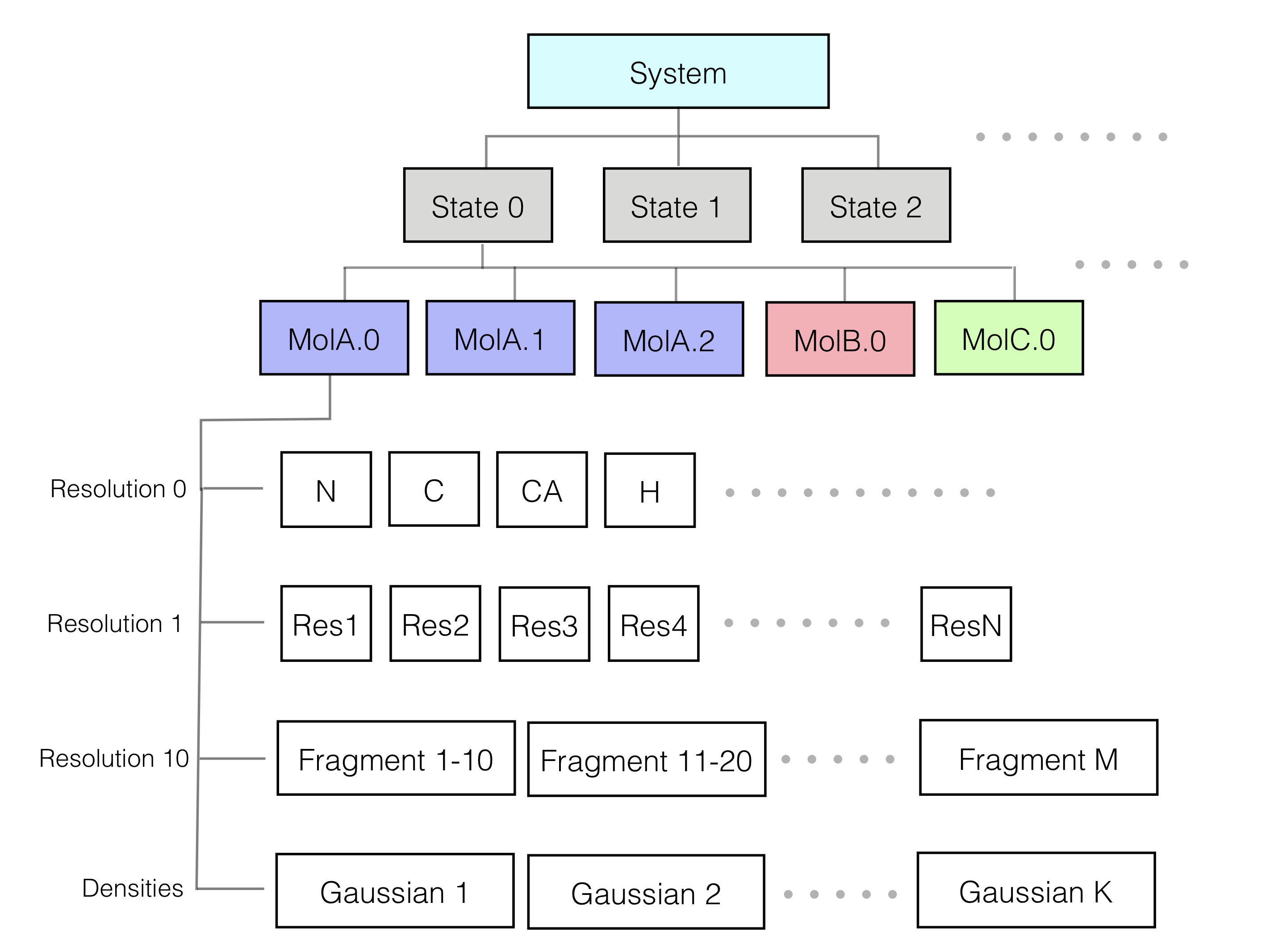
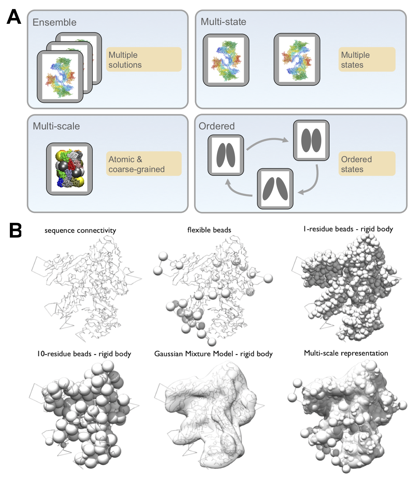
The representation of the system defines the structural degrees of freedom that will be sampled and is designed based on the information at hand. We can utilize a multi-scale representation, where model components can be modeled at one or more different resolutions commensurate with the information content at that site. For example, a domain described by a crystal structure can be represented at atomic resolution and a disordered segment can be represented as a string of spherical beads of 10 residues each. In addition, non-particle based representations, such as Gaussian mixture models (GMMs), can also be used; for example, in EM density fitting. Choosing a representation reflects a compromise between the need for details required by the biological application of the model and the need for coarseness required by limited computing power.

PMI Hierarchy: PMI is constructed as a top-down hierarchy beginning with a System. A system can contain one or more states with each state being a different conformation, composition or time-ordered step in the system. Each state is comprised of one or more molecules that may have one or more copies per molecule. At the final level, each molecule is represented at one or more resolutions.

Some of the input information is translated into restraints on the structure of the model. These spatial restraints are combined into a single scoring function that ranks alternative model configurations (models) based on their agreement with the information. The scoring function defines a multi-dimensional landscape spanned by the model degrees of freedom; the good-scoring models on this landscape satisfy the input restraints.

Ways of representing a single biomolecule: A: The complexity of a molecular system can be represented in four ways. An ensemble of states describes the structural heterogeneity around a single solution. Multiple states are used to describe systems that exist in multiple thermodynamic wells. The system can be modeled at a multitude of scales commensurate with the different types of information known about it. Finally, individual states can be time-ordered, allowing for the modeling of the transition rates between them. B: Multiple representations can be simultaneously applied to the same biomolecule so that information of various types can be applied at the proper scale and form. The molecule is first defined by its sequence connectivity. Flexible beads comprising one or more residues are commonly applied to loops where no high-resolution structure is available. Areas that have high resolution structure can be modeled by spherical beads of 1 residue for the evaluation of residue-specific information such as chemical crosslinks or NMR distance restraints. 10-residue beads are generally used to model lower resolution information such as SAXS data and the excluded volume restraint. The molecule can be represented as a Gaussian mixture model for comparisons to EM densities. IMP and PMI can utilize all of these representations simultaneously in a multi-scale model.

Sampling

In most cases, all possible models cannot be generated. Thus, we utilize sampling methods to search for models that agree with the input data according to the scoring function defined above (good-scoring models). One approach for sampling models in IMP is a Monte Carlo algorithm, guided by our scoring function and accelerated via replica exchange. Other sampling methods can be utilized for specific cases.

Note: Other sampling methods include Rapidly Exploring Random Trees (RRT) for searching dihedral space, divide-and-conquer message passing methods for large discrete spaces, conjugate gradients and molecular dynamics.

Analysis

The results of stochastic sampling (i.e., an ensemble of output structures and their respective scores) must be analyzed to estimate the sampling precision and accuracy, detect inconsistencies with respect to the input information, and suggest future experiments. We wish to analyze only models that are sufficiently consistent with the input information (good-scoring models). A good-scoring model must sufficiently satisfy every single piece of information used to compute it; therefore one needs a threshold for every data point or set of data. Sampling may produce zero such models, which can result from inconsistent data or an unconsidered multiplicity of conformational states (in this case, the user may reformulate the representation by adding a state to the system).

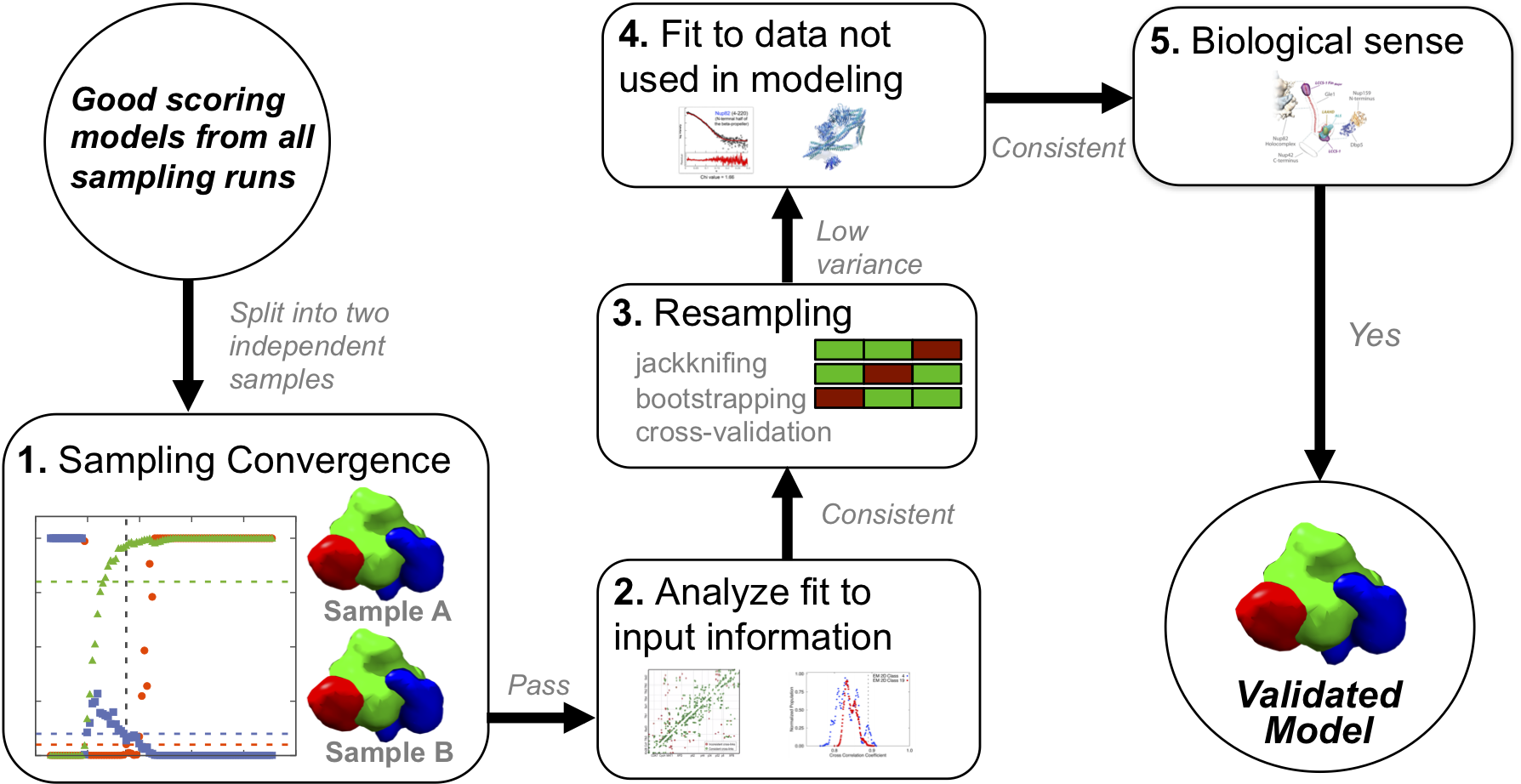
Analysis pipeline: Analysis of sampling runs begins by filtering models that satisfy all input information. In step one, this set is split into two independent samples to assess the precision at which sampling is converged. If sampling has converged at a high enough precision, the resulting models can be assessed against the input information to identify potential multiple states. Resampling can be performed by either systematically or randomly excluding data sets and rerunning the simulation and sampling convergence algorithms. The models can then be assessed against data that was not used in modeling. Finally, the models are assessed for logical sense in answering the original biological question.

Given a set of good-scoring models, we must first estimate the precision at which sampling found these most good-scoring solutions (sampling precision). This estimate relies on splitting the set of good-scoring models into two independent samples, followed by comparing them to each other using four independent tests:

convergence of the model score
whether model scores for the two samples were drawn from the same parent distribution
whether each structural cluster includes models from each sample proportionally to its size
sufficient similarity between the localization densities or the entire system, from each sample.

Note: In general, an ensemble of models can be visualized as a localization probability density map (localization density). The map specifies the probability of any volume element being occupied by a given bead in superposed good scoring models.

After threshold clustering of models, the sampling precision is defined as the largest RMSD value between a pair of structures within any cluster, in the finest clustering for which the structures from the two independent runs contribute proportionally to their size. In other words, the sampling precision is defined as the precision at which the two independent samples are statistically indistinguishable. The individual clusters for each sample are also compared visually to confirm similarity.

At this step, the model precision (uncertainty), which is represented by the variability among the good-scoring models, is also reported. This uncertainty can be quantified by measures such as root-mean-square deviation (RMSD) of model components for models within each cluster or between clusters determined above. The lower bound on model precision is provided by the sampling precision; the model precision cannot be higher than the sampling precision.

An accurate model must satisfy all information about the system, and this is evaluated in a number of steps. First, the consistency of the model with input information is assessed by independently assessing the clusters determined above against the input data. In the next step, the models are assessed by random or systematic cross-validation. The next and most robust validation is the consistency of the model with data not used to compute it, similar to a crystallographic R_free.

A final validation is the presence of features in the model that are unlikely to occur by chance and/or are consistent with the biological context of the system. For example, a 16 fold symmetry was found in the model of the Nuclear Pore Complex when only 8-fold symmetry had been enforced and the displacement of the aspartate sensor domain in a two state model of the histidine kinase PhoQ transmembrane signaling agreed with previous analysis.

A key feature of the four-step procedure for integrative modeling is that it is iterative. Assessment may reveal a need to collect more input data, or suggest future experiments, both by the researchers that constructed the initial model and by others.

Deposition

For the models, data, and modeling protocols to be generally useful, they must be reproducible and available to everyone in a publicly accessible database. This availability allows any scientist to use a deposited model to plan experiments by simulating potential benefits gained from new data. Computational groups can more easily experiment with new scoring, sampling, and analysis methods, without having to reimplement the existing methods from scratch. Finally, the authors themselves will maximize the impact of their work, increasing the odds that their results are incorporated into future modeling. Following the recommendations of the wwPDB Hybrid/Integrative Methods Task Force in 2015, a new archive, PDB-IHM was established to store integrative models and corresponding data. The mmCIF file format used to archive regular atomic PDB structures was extended to support the description of integrative models, including information on the input data used, the modeling protocol, and the final output models. As of December 2024, PDB-IHM contains 339 depositions, including 55 generated by IMP.

Next, on to modeling of the actin-tropomodulin-gelsolin complex.

Table of Contents