 |
|
Modeling of an actin complex with PMI
|
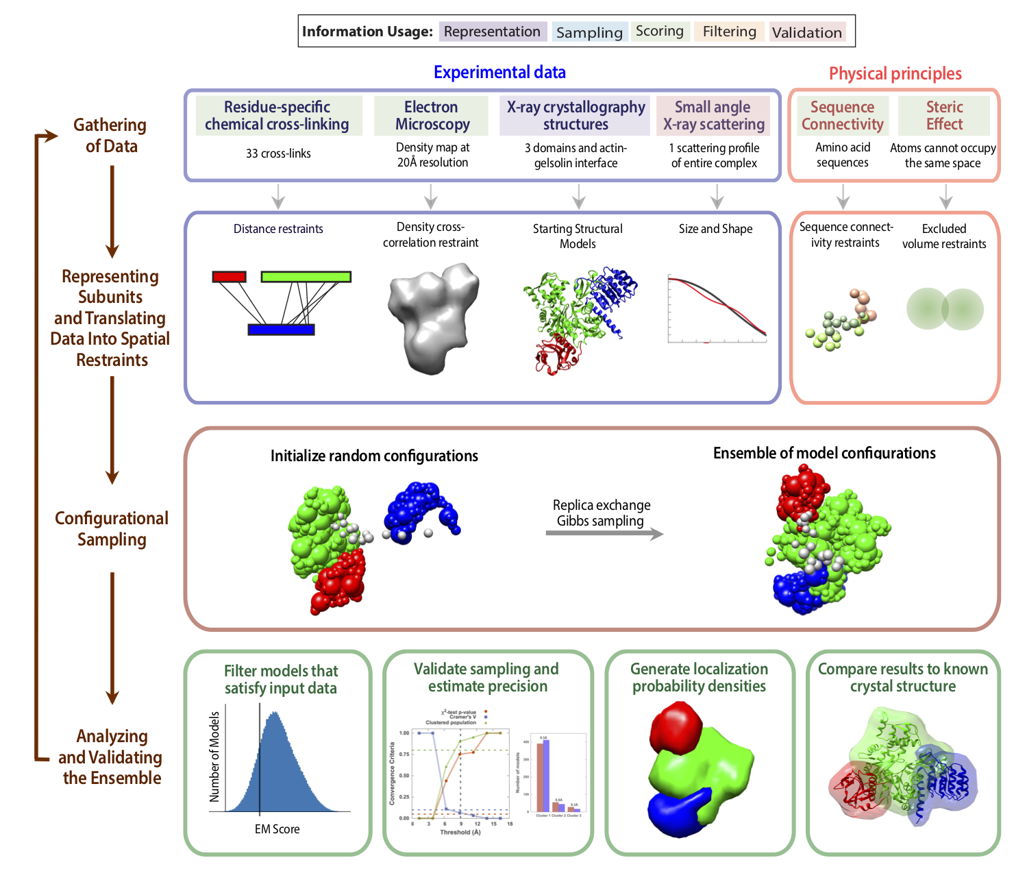
Here, we demonstrate integrative modeling using the PMI interface by modeling the complex of actin and tropomodulin-gelsolin chimera using SAXS, EM, crosslinking, crystal structures of the individual domains, and physical principles. This complex was solved via X-ray crystallography at 2.3 Å resolution (PDB: 4PKI). We use this structure to simulate biophysical data and assess the accuracy of the modeled complexes. In this simple exercise, we assume that we have a crystal structure of only the actin-gelsolin interface and would like to find the tropomyosin-actin binding interface. The entire modeling protocol is summarized in the four-stage diagram below:
To follow this tutorial, first download the data files, either by cloning the GitHub repository or by downloading the zip file.
All data is contained in subfolders of the data directory of the tutorial.
The crystal structure 4PKI is used to set the atomic coordinates for each of the domains in the FASTA sequence that determines the composition of each biomolecule as well as the coordinates for tropomyosin and the actin-gelsolin complex.
Thirty-three simulated crosslinks were generated from a random subset of lysine residues whose CA-CA distances are under 25 Å.
A simulated EM density of the entire complex was created at 20Å resolution using IMP. The simulated map is approximated as a Gaussian Mixture Model (GMM).
simulate_density_from_pdb <file.pdb> <output.mrc> <resolution> <a/pixel>A simulated SAXS profile of the entire 4pki.pdb complex was created using FoXS.
We also define restraints such as excluded volume and sequence connectivity to add chemical and physical knowledge to the modeling protocol.
The model representation (e.g., bead size and rigid bodies) can be set within the topology file. The topology file is a pipe-delimited format with each line specifying a separate domain and keyword values determining how the domain is represented. For more information on the topology file and its contents, see the PMI documentation.
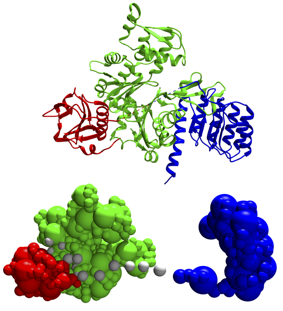
The topology file for this tutorial, shown below, is found at modeling/topology.txt. Here, the system is subdivided into four distinct domains: one each for the three structured domains (actin, gelsolin, and tropomyosin) and one consisting of the 18-residue engineered linker between gelsolin and tropomyosin. The first domain, the entire actin molecule, is colored green and contains the entirety of chain A from 4pki.pdb. A bead_size of 1 residue per bead is assigned to any unmodeled section, i.e. not present in the PDB file (spherical beads are applied to every 10 residues with smaller beads applied to loops of smaller length). A GMM is approximated using 10 residues per Gaussian. This domain is assigned to rigid_body 1. The second domain, the gelsolin portion of the chimera, is constructed by selecting the residue_range 52-177 of chain G. These residues, however, are numbered 1-126 in the FASTA file, therefore a pdb_offset of -51 must be added. This domain is also assigned to rigid_body 1 to preserve the actin/gelsolin interface. The third domain is the linker, whose residues have no structure associated with them; thus, they are given a pdb_fn of BEADS with a bead_size of 1 (these residues are also assigned to rigid_body 1 to improve sampling; all beads within rigid bodies are, by default, allowed to be flexible). The final domain, tropomyosin, is built similarly to gelsolin and assigned to rigid_body 2, since we would like to sample its position separate of the rest of the complex.
This topology file also places all domains in a single super_rigid_body. This definition allows the entire complex to move as a single unit, which is useful for fitting to the EM map.
The modeling script contains the entire workflow from defining the system representation through execution of sampling. The system representation and sampling degrees of freedom can be built manually or, as here, read from a topology file. Restraints are added, and the sampling protocol defined and executed.
modeling/modeling_manual.py contains this exact system built manually using PMI commands instead of a topology file. PMI commands allow significantly more flexibility in model design.First, we create an IMP Model object, which stores all components of the model. Second, we create a BuildSystem object and define the resolutions at which residues in the structured sections will be modeled. Here, we set resolutions of 1 and 10 residues per bead so that crosslinking restraints can be evaluated at residue resolution and the expensive excluded volume restraint (below) can be evaluated at the lower resolution. Third, the topology file is read using a TopologyReader object, followed by generating a useful list of component molecules. To this BuildSystem object, we add a state corresponding to the representation defined in the topology file using bs.add_state().
bs.add_state(t2) can be invoked with a different topology file.We then execute the macro, which returns the root_hier root hierarchy and dof degrees of freedom objects, which will be used later. Within the macro, we set the movement parameters of individual beads and rigid bodies. Translations (trans) are defined in angstroms and rotations (rot) in radians:
PMI contains simple interfaces for a number of IMP restraints that model various types of chemical and physical data and knowledge. All of these restraints produce output, which we will collect in an output_objects list. Each restraint also needs to be explicitly added to the scoring function for sampling,using the add_to_model() command. We will add the restraints to the scoring function in a specific order, discussed below. First, we define the restraints that enforce physical and chemical principles. (For coarse-grained models, a molecular mechanics forcefield is not applicable. The CHARMM force field can be applied to enforce stereochemistry on atomic models, however. See the examples in the IMP.atom module to learn how to implement this restraint.)
The ConnectivityRestraint adds a bond between each pair of consecutive residues in each molecule. The ExcludedVolumeSphere restraint is applied to the entire system and enforced at the lowest resolution possible (indicated by resolution=1000), because this restraint is costly to evaluate:
Second, we build a SAXSRestraint based on the comparison of SAXS data to the model. Since our model is calculated at residue resolution, we calculate the SAXS profile using residue form factors. For residue-based calculations, we compare curves out to a q of 0.15. (Model SAXS profiles can be computed using residues, CA atoms, heavy atoms or all atoms, depending on the resolution of the model. The recommended maxq values are dependent on this choice. At residue resolution, the fit is only valid up until q ~ 0.15; for heavy atoms q = 0.4; and for all atoms, the fit is valid out to q = 1.0 (the maximum value).)
To set up a crosslinking restraint, we first build a PMI CrossLinkDataBase that uses a CrossLinkDataBaseKeywordsConverter to interpret a crosslink data file. At a minimum, the crosslink data file needs four columns labeled with a key: one for each protein name and one for each residue number of the crosslink. The standard keys are Protein1, Residue1, Protein2, Residue2 (see derived_xls.dat and the modeling.py script for a more in-depth explanation of crosslink keys).
Using this database, we can construct the crosslinking restraint. We input the root hierarchy of the system and the database, and specify the length and chemistry of the crosslinker. The restraint can be evaluated at any resolution, though is generally most informative at resolution = 1. The length determines the inflection point of the scoring function sigmoid and is generally set to 10Å+ the crosslinker length for Lys-Lys crosslinkers.
The crosslinker chemistry is not used in the modeling, but it is written into the output file metadata, which can be used for validation or deposition.
The EM restraint is determined by calculating the overlap (cross-correlation) between the system GMM density particles and the map GMM particles. First, we must collect the density particles using an IMP Selection. We then invoke the restraint using these particles and the gmm file generated from the EM map.
Sampling begins by randomizing the coordinates of the starting particles using shuffle_configuration. Because this randomization generally places beads of neighboring residues far apart, we first optimize the positions of these flexible beads using steepest descent minimization for 500 steps based on only the connectivity restraint. We then add the balance of the scoring function terms to the model prior to the main sampling step.
max_translation parameter. Don’t set this too high as you’ll spend way too much time getting your system to move back together.We implement a Monte Carlo sampling scheme with replica exchange using the PMI ReplicaExchange macro. Within this macro, we set the directory where all output files will be placed, global_output_directory, and the number_of_frames to generate. The final line of the script executes the sampling macro.
Modeling analysis requires at least two independent sampling runs be performed. For each run, in modeling.py the global_output_directory keyword can be set to run1, run2, ..., runX.
The modeling script can be run on a single processor using the following command:
or in parallel using N processors using:
A parallel invocation of IMP will run replica exchange with N replicas. A serial run will run a basic Monte Carlo protocol with one replica.
Raw output will be written to the runX/output folder, as specified in the replica exchange macro. Within this folder, stat files contain tabulated statistics for each frame. In the rmf directory, model coordinates for the lowest temperature replica are stored. These can be opened directly in UCSF Chimera or ChimeraX and the "trajectories" observed.
Next, on to analysis of the actin complex models and deposition.
