 |
|
IMP Manual
for IMP version 2.16.0
|
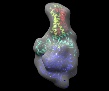
In this example, EMageFit is used to build a model of porcine mitochondrial respiratory complex II (PDB id 3sfd), using crystal structures of its 4 constituent proteins and a number of electron microscopy (EM) class averages of the complex. For more information on the protocol employed during this example, see the EMageFit protocol page.
(See also the MultiFit example for building models using 3D EM maps instead of 2D class averages.)
All steps in the procedure use a command line tool called emagefit. For full help on this tool, run from a command line:
First, obtain the input files used in this example and put them in the current directory, by typing:
(On a Windows machine, use xcopy /E rather than cp -r.) Here, <imp_example_path> is the directory containing the IMP example files. The full path to the files can be determined by running in a Python interpreter 'import IMP.EMageFit; print(IMP.EMageFit.get_example_path('3sfd'))'.
The input files are for modeling are the three simulated class averages of the complex located in the em_images directory, and the subunits to assemble: 3sfdA.pdb, 3sfdB.pdb, 3sfdC.pdb, and 3sfdD.pdb. A number of Python files are also present. These control the modeling procedure and are described below. For an extensive description of all the parameters see config_example.py.
Building a model requires 4 steps: pairwise docking between interacting subunits, SA-MC optimization, SA-MC model gathering, and DOMINO sampling.
To do the dockings, run from the command line:
Open the file dock.log and search for the line:
INFO:buildxlinks:The suggested order for the docking pairs is [('3sfdB', '3sfdA'), ('3sfdB', '3sfdC'), ('3sfdB', '3sfdD'), ('3sfdD', '3sfdC')]
EMageFit has determined the dockings required, and the order recommended. The pairs are (Receptor,Ligand), so 3sfdA should be docked into 3sfdB, and so on. If HEXDOCK is installed, it is used to perform these dockings, and generates several sets of new files. These include PDB files of the initial docking solutions as estimated from the cross-linking restraints (ending in initial_docking.pdb); the PDB files with the best solutions from HEXDOCK (ending in hexdock.pdb); a set of text files starting with hex_solutions, containing all the solutions from HEXDOCK; and 4 text files starting with relative_positions, which contain the relative transformations between the subunits participating in each pairwise docking. This last set of files is used by the SA-MC optimization.
If HEXDOCK is not present, the relative positions files need to be generated using some docking algorithm. They have a simple format; each line is simply the transformation needed to dock the ligand to the receptor, given as the components of the rotation quaternion followed by the translation vector.
Next, the anchor component and the docking transforms need to be placed into the configuration file for the next step, by setting self.anchor and self.dock_transforms respectively. The anchor component is the component with most neighbors, and is the first receptor in the list of docking pairs printed in the log file (the second component, 3sfdB, in this case). (Anchored components are not moved during the SA-MC optimization.) The file config_step_2.py includes this information.
The next step is running a Monte Carlo optimization. There are several parameters to control this optimization, such as the profile of temperatures, number of iterations, cycles, maximum displacement and angle tolerated for the random moves, and also the parameter self.non_relative_move_prob. This last parameter indicates the probability for a component of undergoing a random move instead of a docking-derived relative move. For example, a value of 0.4 means that the component acting as ligand (e.g. 3sfdA) will prefer to do a random move with respect to its receptor (3sfdB) 40% of the time. A value of 1 ignores all the relative positions, and a random move is always chosen (i.e. all docking solutions are ignored). To run the optimization:
Note that config_step_2.py sets Monte Carlo parameters to get a very short simulation, for demonstration purposes. For serious application, a longer Monte Carlo simulation is recommended; suitable parameters can be found in config_step_1.py.
The output is the file mc_solution1.db, an SQLite database with the solution. To generate multiple candidate solutions, simply run the command multiple times with different output file names.
After generating a set of solutions, they must be gathered together into a single database, using a command such as:
For this example, a pre-built database is included in the outputs directory, containing the results of 500 Monte Carlo runs. To use this for subsequent steps in the example, run:
The last part of the modeling is running DOMINO employing the configuration file config_step_3.py. This new configuration file has changes with respect to config_step_2.py in the classes DominoSamplingPositions and DominoParams. The parameters are:
self.read is the file with the Monte Carlo solutions obtained before.self.max_number is the maximum number of solutions to combine. In this example, with 500 solutions and 4 components, strict enumeration would require 5004 combinations to be explored, which is unfeasible. This number allows you to reduce that. In this example, it is set to 5, and therefore only 54 combinations are explored.self.orderby is the name of the restraint used to sort the Monte Carlo solutions. Here the value is "em2d", so the best 5 solutions according to the em2d score will be combined with DOMINO. Another option is to use "total_score".self.heap_solutions. This is a rather technical parameter. It is the number of solutions that DOMINO keeps at each merging step. The larger the number, the better the space of 54 combinations is explored, at the cost of a larger running time. Here, a value of 200 is used.The command to run is:
The output domino.db is a database of solutions. For the actual benchmark used in the EMageFit publication, parameters of self.max_number=50 and self.heap_solutions=2000 were used, resulting in the file outputs/domino_benchmark.db.
The solutions can be written out as PDB files. To write out the 10 best models according to the value of the em2d restraint, run:
The best solution, shown fitted in the density map of the complex, is shown below: