 |
|
IMP Manual
for IMP version 2.9.0
|
In the analysis stage we cluster (group by similarity) the sampled models to determine high-probability configurations. Comparing clusters may indicate that there are multiple acceptable configurations given the data.
A long modeling run was precomputed and analyzed. You can download it from our website, and you can download the corresponding analysis.
The clustering.py script, found in the rnapolii/analysis directory, calls the AnalysisReplicaExchange0 macro, which finds top-scoring models, extracts coordinates, runs k-means clustering, and does basic cluster analysis including creating localization densities for each subunit. The script generates a directory containing as many subdirectories as the number of clusters queried. Each subdirectory contains an RMF and a PDB for each structure extracted, a stat file, and the localization densities.
We can choose the number of clusters, the subunits we want to use to calculate the RMSD, and the number of good-scoring solutions to include. These options are at the top of the script:
If we perform sampling multiple times separately, they can all be analyzed at the same time by appending to merge_directories. The prefiltervalue removes all models scoring below this value (meaning, they aren't clustered) which can be helpful to reduce the problem size.
Create the analysis macro and pass it basic information (it will search for stat files):
These are features that are kept around (and moved to the cluster stat files):
Now we specify the subunits (or groups or fractions of subunits) for which we want to create density localization maps. density_names is a dictionary, where the keys are convenient names like "Rpb1-CTD" and the values are a list of selections. The selection items can either be a domain name like "Rpb1" or a list like (200,300,"Rpb1") which means residues 200-300 of component Rpb1. This enables the user to combine multiple selections for a single density calculation.
Next, we specify the components used in calculating the RMSD between models. All selections here are used together for a single RMSD calculation between two models. The format is the same as density_names. One use case is when only a subset of the system is actually being sampled (with the rest kept static). Note that unless you provide something to align_names (see below), no alignment is done before calculating RMSD.
Next, we specify components used for structural alignment. This is needed in case there is no absolute reference frame (like an EM map). The format is the same as density and RMSD. In this case we use None because of the EM map.
Finally, we start the clustering. Most of the options were chosen earlier in the script.
Run the clustering script by changing into the rnapolii/analysis directory and then running:
If you ran modeling.py with the --test option, it is a good idea to give the --test option to clustering.py as well (this increases the prefilter value; none of the 50 test models generated may be good enough to satisfy the default prefilter value). With such minimal sampling, the quality of the results is unlikely to be high; you can download the precalculated results and the resulting clusters from our website.
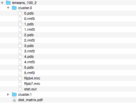
First we can look through the cluster results directory to see the output (see example below). The clustering directory contains the distance matrix plot (described below) and a folder for each cluster. Within the cluster folder are PDB and RMF files containing members of each cluster, localization densities for requested components (the .mrc files), and a stat file output (with one entry for each cluster member). All RMF, PDB, and MRC files should be viewable in Chimera.
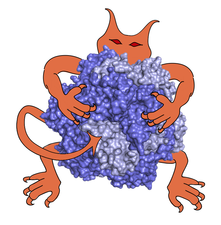
Here is an example modeling result (from the provided files, cluster.1/4.rmf3, the cluster center):
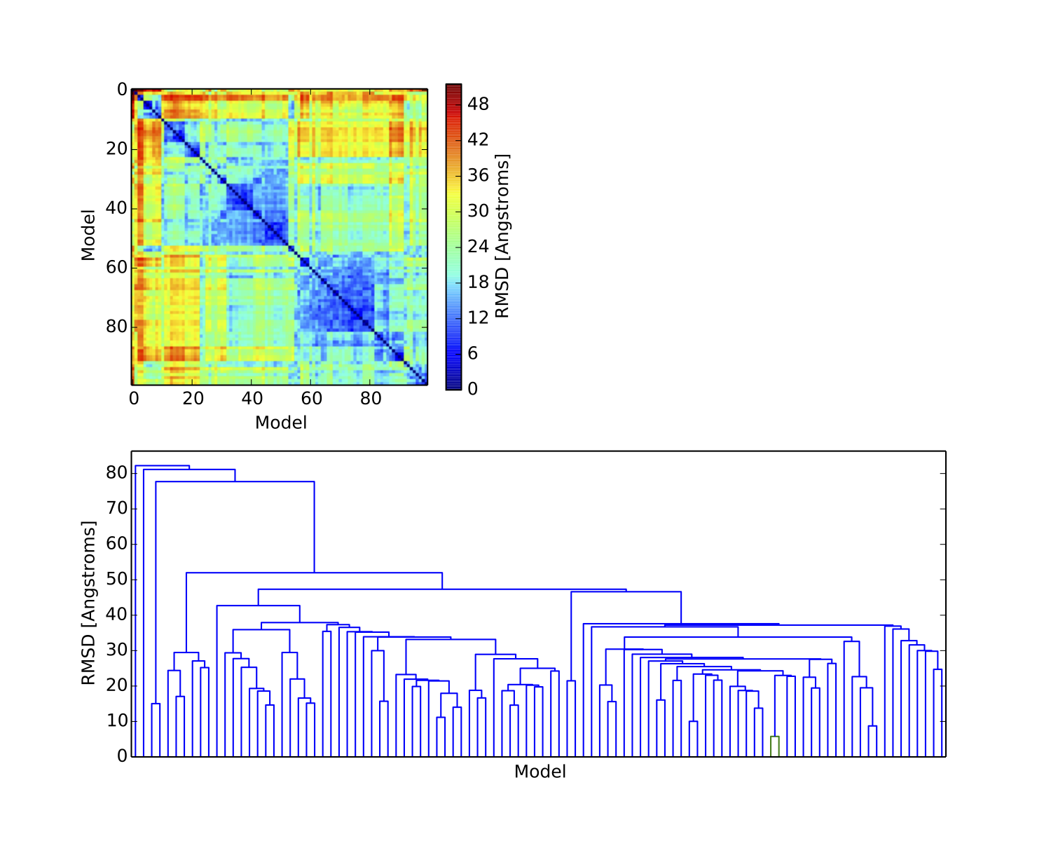
Next we can examine the plots outputted by the clustering script. The plots are output to a single file (dist_matrix.pdf) in the clustering directory. The first plot is the distance matrix of the models after being grouped into clusters. The matrix should show the requested number of clusters with much lower within-cluster than between-cluster distance. If this is not the case, then perhaps too many clusters were chosen.
The second plot is a dendrogram, basically showing the distance matrix in a hierarchical way. Each vertical line from the bottom is a model, and the horizontal lines show the RMSD agreement between models. Sometimes the dendrogram can indicate a natural number of clusters, which can help determine the correct number to use. Here is the result from using 2 clusters on the example results:
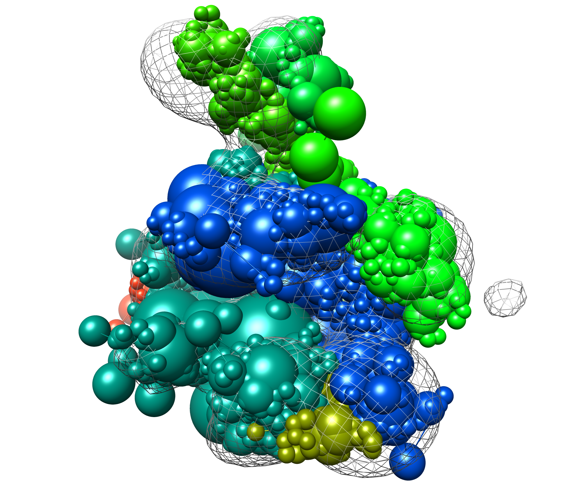
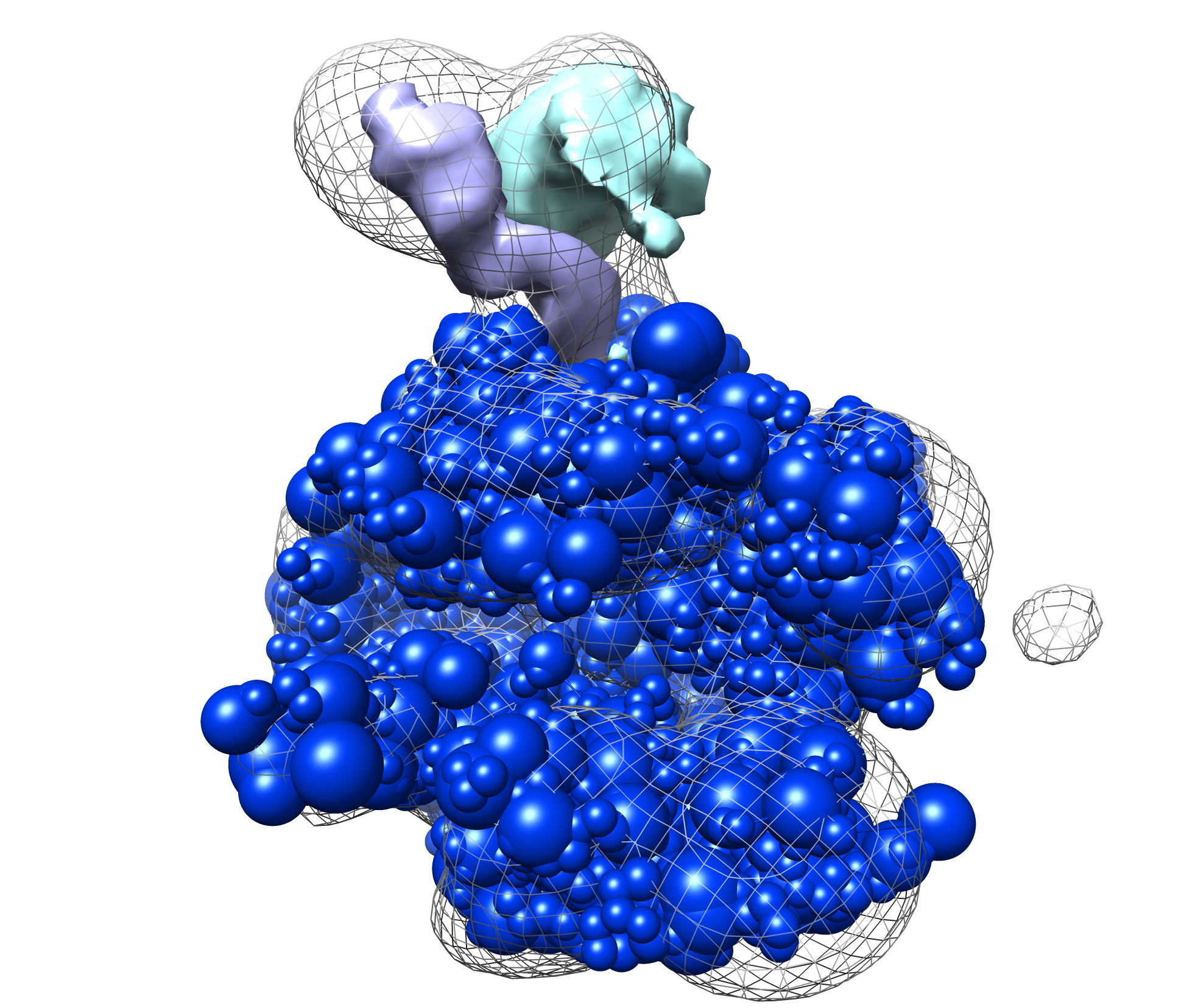
Next can examine the localization densities of a cluster. These can give a qualitative idea of the precision of a cluster. Below we show results from cluster.1 in the provided results: the native structure without Rpb4/7 (in blue), the target density map (in mesh), and the localization densities (Rpb4 in cyan, Rpb7 in purple). The localizations are quite narrow and close to the native solution:
For quantitative analysis of the clustering results we need to call another script (see Part 2).